Issues with Sketchmap Loss
In recent years Deep Learning has become ubiquotus in science and many fields have started using Deep Learning techniques in order to analyze data. One such way is to use an Autoencoder network in order to reduce the dimensionality of some data to extract structures otherwise invisible.
The Encodermap architecture does exactly that. By adding a second loss term based on the Sketchmap loss, the architecture not only reduces dimensionality, but also keeps some interesting structure from the fine-grained data.
The idea is that, by training with both the standard loss and the Sketchmap loss, the Encodermap architecture can learn to encode the data in a way that is both low-dimensional and sensitive to the important details in the data. This is especially helpful for data where long range dependencies are not of interest, and short range dependecies can be noisy.
But while experimentally producing good results, the Sketchmap loss used has bad sensitivity when used as a loss that produces gradients.
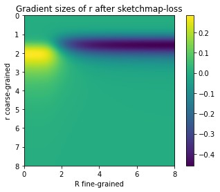
This is because gradients vanish when the coarse values are not in the chosen medium regime, leading to no effective update when coarse values are too high or too low, even though the fine-grained values are in the medium regime.
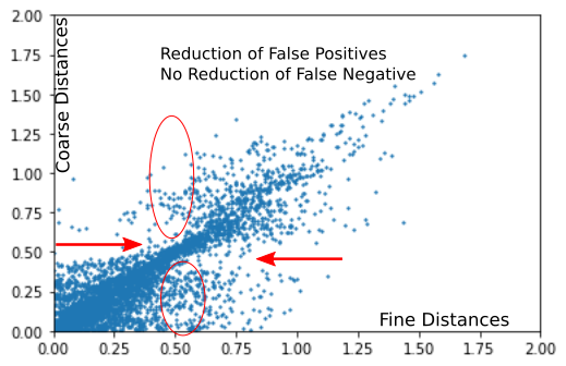
Effectively this means that Sketchmap Loss reduces the number of false positives (i.e. coarse prediction is medium when it shouldn’t be) but does nothing against false negatives (i.e. coarse prediction is high or low when it shouldn’t be).
In practice this is often irrelevant, as the Autoencoder is strong enough to mitigate these differences, and some false negatives do not impact the encoding too much. The problem does however still exist, and one should be aware of this issue when using Sketchmap Loss in gradient based methods.
Sketchmap Loss
The Sketchmap Loss is defined as the squared distance between the sigmoids of two distance matrices.
\[C_{sketch} = \frac{1}{m} \sum_{i\neq j} [SIG_h(R_{ij})-SIG_l(r_{ij})]^2\](see here)
Where $SIG$ describes a sigmoid function of the form
\[SIG_{a,b,\sigma}(r) = 1-(1+(2^{a/b}-1)(r/\sigma)^a)^{-b/a}\]$\sigma$ determines the inflection point of the sigmoid function. Note that $SIG_{a,b,\sigma}(0)=0$, $SIG_{a,b,\sigma}(\sigma)=0.5$ and $lim_{r \rightarrow \infty} SIG_{a,b,\sigma}(r)=1$
The loss $C_{sketch}$ is 0 exactly when $R_{ij} = r_{ij}$ and differences from this equality are weighted more strongly at the inflection point. Note that it does not matter if $R$ or $r$ is close to the inflection point, as the loss is symmetric in $R$ and $r$.
This is not the case when using it as a gradient producing approach to optimize $r$. As we calculate the gradient by calculating the derivative fo $r$, we break symmetry and $r$ and $R$ have different influences.
The sketchmaploss has the following property:
\[\frac{\partial C_{sketch}}{\partial r_{ij}} = \frac{\partial SIG_l(r_{ij})}{\partial r_{ij}}\cdot 2 \cdot (SIG_h(R_{ij})-SIG_l(r_{ij}))\]As the $SIG$ function quickly saturates when moving away from the inflection points it follows that:
\[\frac{\partial C_{sketch}}{\partial r_{ij}} \rightarrow 0 \text{ as } |r_{ij} - \sigma_r| \rightarrow \infty\]So, as our distance from the inflection point increases, the gradient goes towards 0. At first glance this seems fine, but this leads to an issue. It is enough for the $r$ values to strongly differ from the inflection point to completely stop any sketchmap gradient from occuring. In particular, this means that it is irrelevant if the $R$ values are close to the inflection point or not. The strength of the gradient depends mostly on the $r$ values.
So we get the following table:
| Coarse is Medium-Distance | Coarse is not Medium-Distance | |
|---|---|---|
| Fine is Medium-Distance | Good | Bad and doesn’t udate |
| Fine is not Medium-Distance | Bad, but will update | Good |
In classical Machine Learning this corresponds to a False Negative Error.
What does this effectively mean? It means that medium distance dependencies are not necessarily captured, quite the contrary: Non medium distances are captured!
Note that this is an artifact of using the Sketchmap Loss to calculate a gradient. The global minimum of the loss does fit medium to medium distances. It is however not effectively reachable by gradient descent.
Experiments
Optimizing only the sketchmap loss on data leads to the behavior predicted above. We sample some high dimensional and low dimensional points and try to optimize the pairwise distances in the low dimensional regime to fit those of the high dimensional regime using sketchmap loss.

Every point in the graphic can only move vertically, as the fine (high dimensional) distances are fixed. As we can see, optimizing the sketchmap loss does not effectively reduce the number of False Negatives, while False Positves are handled very well.
Designing a more fitting loss function
If we investigate the Gradients of the above loss as a 2D Image, they look like this:

Showing Gradients along only a single axis, in concordance to the above plot.
We want to symmetrize this somewhat. As shown above these gradients are described by:
\[\frac{\partial C_{sketch}}{\partial r_{ij}} = \frac{\partial SIG_l(r_{ij})}{\partial r_{ij}}\cdot 2 \cdot (SIG_h(R_{ij})-SIG_l(r_{ij}))\]A better Gradient would look like this:
\[\frac{\partial C_{sketchBetter}}{\partial r_{ij}} = (\frac{\partial SIG_l(r_{ij})}{\partial r_{ij}}+ \frac{\partial SIG_h(R_{ij})}{\partial R_{ij}})\cdot 2 \cdot (SIG_h(R_{ij})-SIG_l(r_{ij}))\]Which can be rewritten as:
\[\frac{\partial C_{sketchBetter}}{\partial r_{ij}} = \frac{\partial C_{sketch}}{\partial r_{ij}} + \frac{\partial SIG_h(R_{ij})}{\partial R_{ij}}\cdot 2 \cdot (SIG_h(R_{ij})-SIG_l(r_{ij}))\]The loss should then be given by
\[C_{sketchBetter} = C_{sketch} + 2\cdot \frac{\partial SIG_h(R_{ij})}{\partial R_{ij}} \cdot SIG_h(R_{ij})\cdot r_{ij} - 2\cdot \frac{\partial SIG_h(R_{ij})}{\partial R_{ij}} \cdot\int SIG_l(r_{ij}) dr_{ij} + const.\]$const.$ should be irrelevant as we only care about the derivative(?)
$\frac{\partial SIG_h(R_{ij})}{\partial R_{ij}}$ is easy to calculate, the only issue is $\int SIG_l(r_{ij}) dr_{ij}$, which does not possess a simple closed form.
We might get away with replacing the Integral with some fake function that has the right properties. As the SIG function saturates to (0?) and 1, this might be some sort of SELU function.